If you can't find the product or version you're looking for, visit support.ataccama.com/downloads

Anomaly Detection in Catalog Items

Potential anomalies are detected during the profiling of catalog items on two levels:

Catalog item level, on metrics such as number of records, summary statistics, and so on.
Attribute level, on metrics such as value distribution, standard deviation, numeric sum.

The value of the metric is considered to be an anomaly if it is beyond the usual range. Anomaly detection is a process handled with AI, meaning that with every confirmed or dismissed alert, ONE learns more about the data and its possible values, which helps in detecting anomalies more precisely with every profiling.

The anomaly detection feature in the Data Catalog behaves differently based on the settings you select.

There are two key properties you can configure in the profiling settings:

Type of model: This option allows you to select the type of model to use for anomaly detection. You can choose between a time-dependent or time-independent model.

Determining which model is appropriate for your use case is key.
Degree of sensitivity: By default, the anomaly detection sensitivity is set to medium. However, depending on the desired behavior, you can adjust this setting to increase or decrease how far a value needs to be from the expected value to be considered an anomaly.

The models also have adaptive sensitivity: in the beginning it tends to be less sensitive, because the algorithm needs to learn what is considered usual behavior.

Configuration of these settings is covered in Time-independent vs. time-dependent model and Anomaly detection sensitivity respectively, but if you are not sure yet which settings might best suit your use case, see How do I get anomaly detection to work for me?.

Time-independent vs. time-dependent model

It’s important to select the correct model for your data: for example, the time-independent model is not ideal when a trend is present; it’s much better to use the time-dependent model.

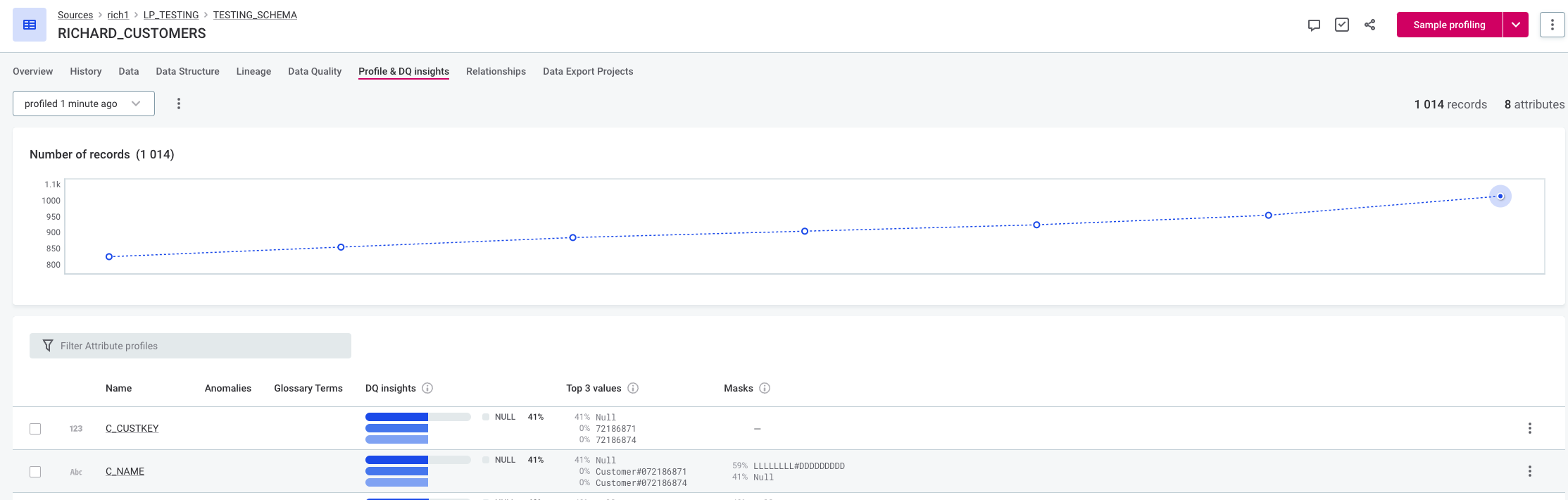
The following figure shows the time-independent model with medium sensitivity. It can’t model the trend and detects an anomaly when the increase is higher than previous increases.

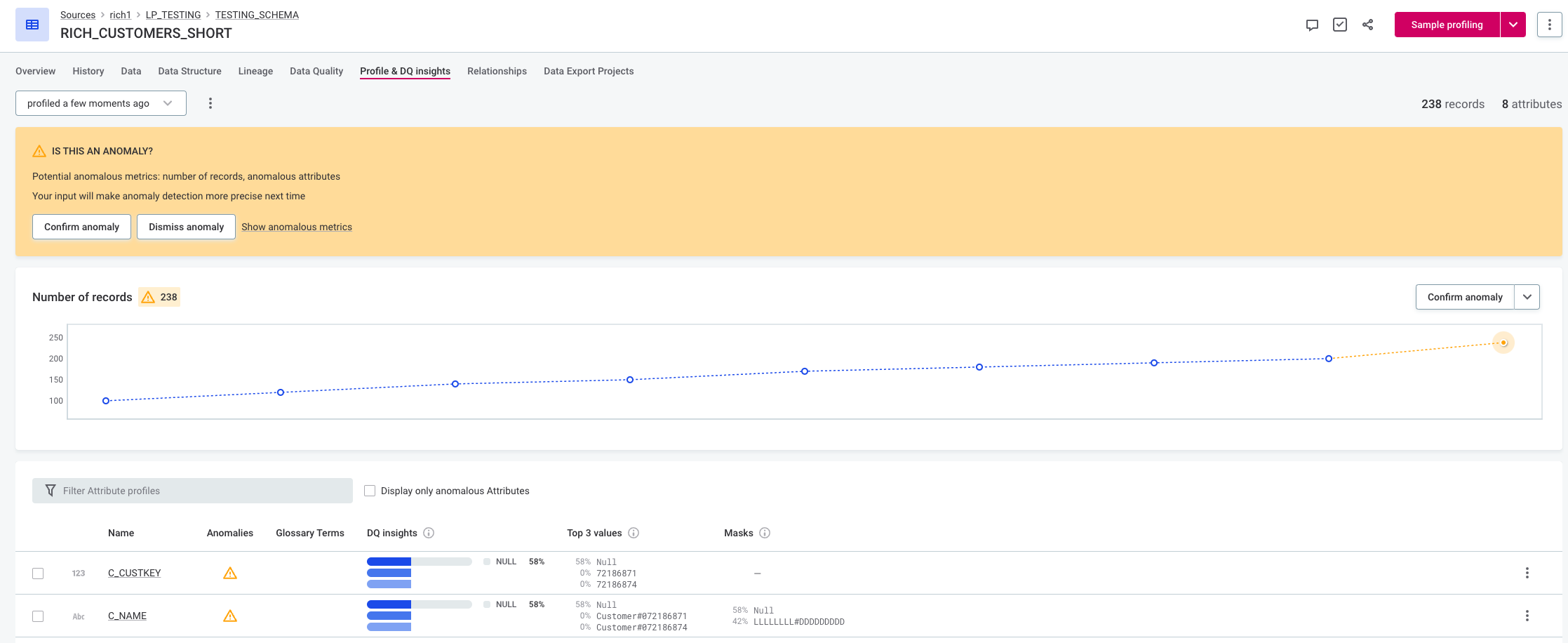
If you do choose to use the time-independent model in this scenario, the results can be slightly improved by using a lower sensitivity setting.

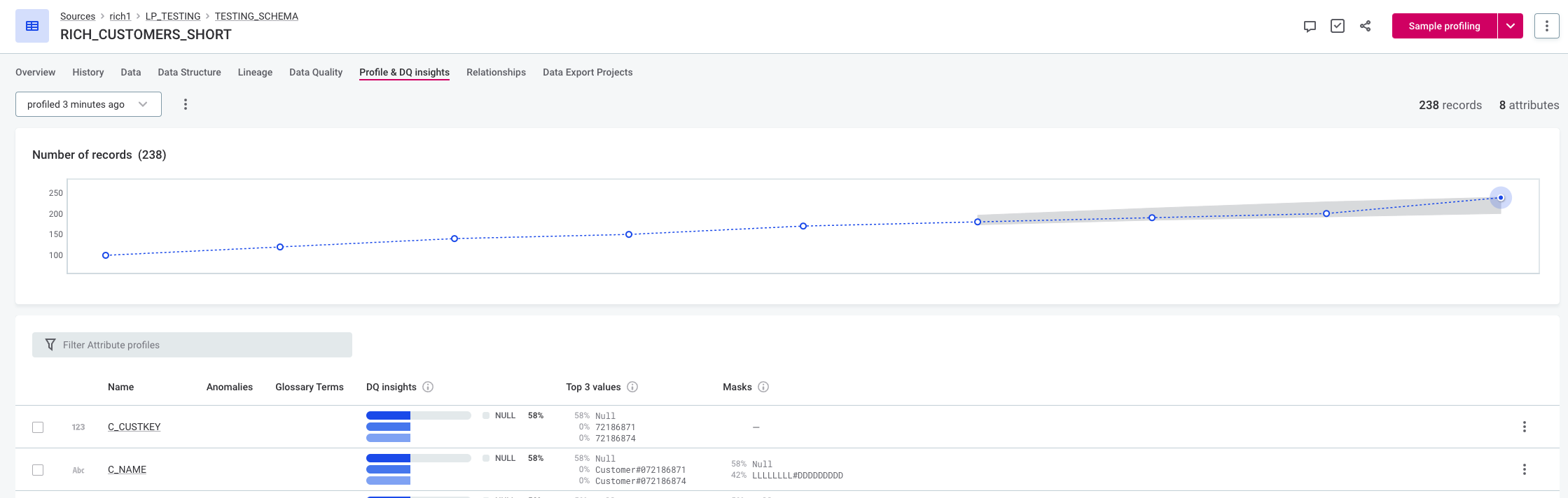
Time-dependent model with medium sensitivity can capture the trend and does not flag the increase as anomalous.

Keep in mind that if you select time-dependent anomaly detection, the periodicity is 1 by default, meaning the general trend of the data is modelled. If you need to account for seasonality instead, you can do this from a monitoring project. To get started with monitoring projects, see Monitoring Projects.

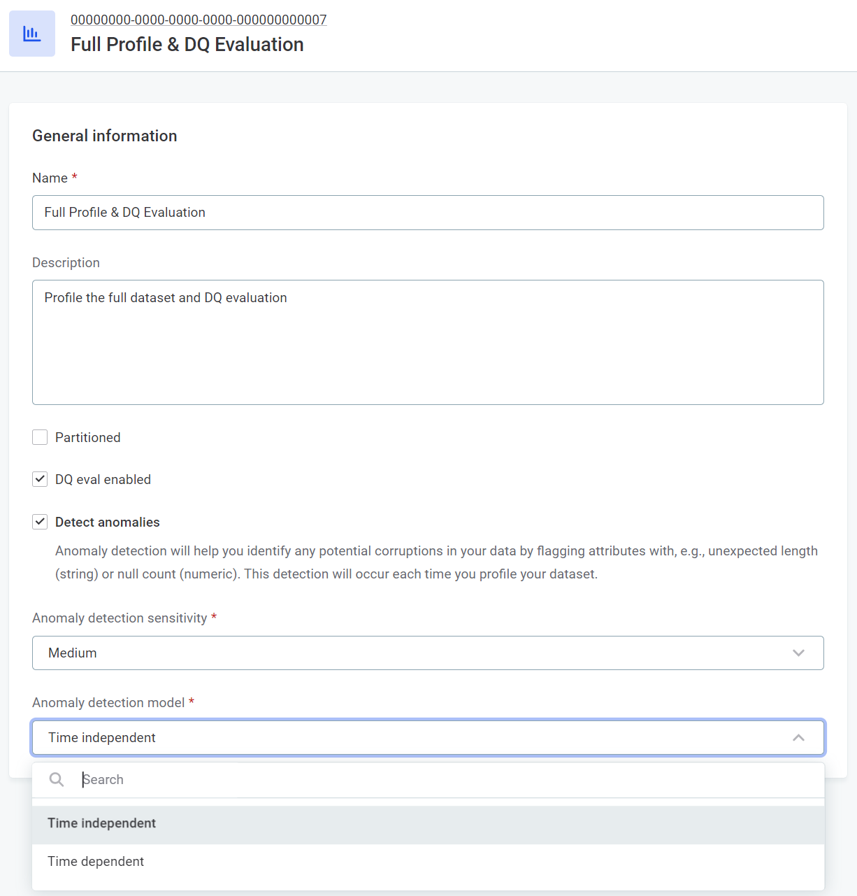
To select the model you want to use in profiling:

Select Global Settings > Profiling, and after selecting the required profiling configuration, select Edit.
In Anomaly detection model, select Time independent or Time dependent.

The minimum required number of runs for both time-independent and time-dependent anomaly detection is six.

More information about the models can be found in Anomaly Detection: Behind the Scenes.

Anomaly detection sensitivity

It is very important to set the appropriate anomaly detection model sensitivity for your data depending on how cautious you want your approach to anomalies to be:

Higher sensitivity produces more anomaly warnings, detecting even minor variations from the previously observed behavior of your data.
Lower sensitivity produces warnings only about very significant variations, leading to fewer anomaly warnings.

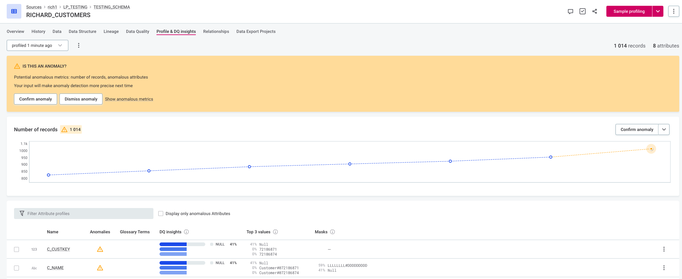
Compare the following figures with different sensitivity settings for the time-independent model. With high sensitivity, the last value is detected as anomalous due to it being out of the previously observed range. With medium sensitivity the last value is not detected as anomalous.

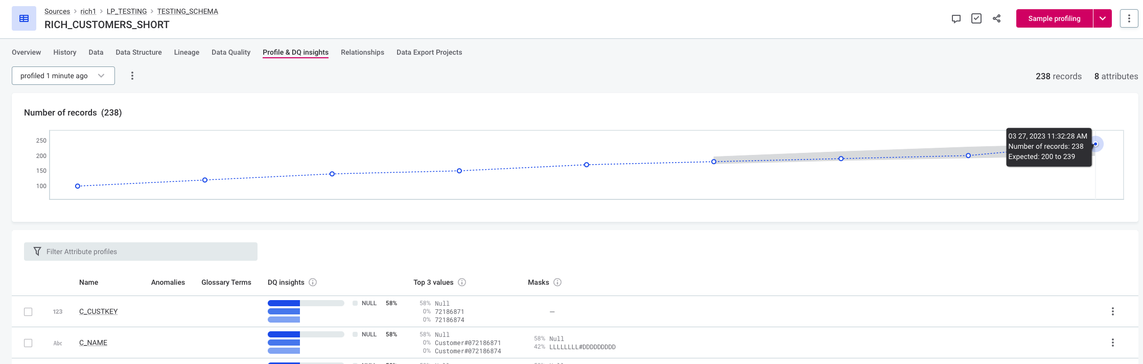
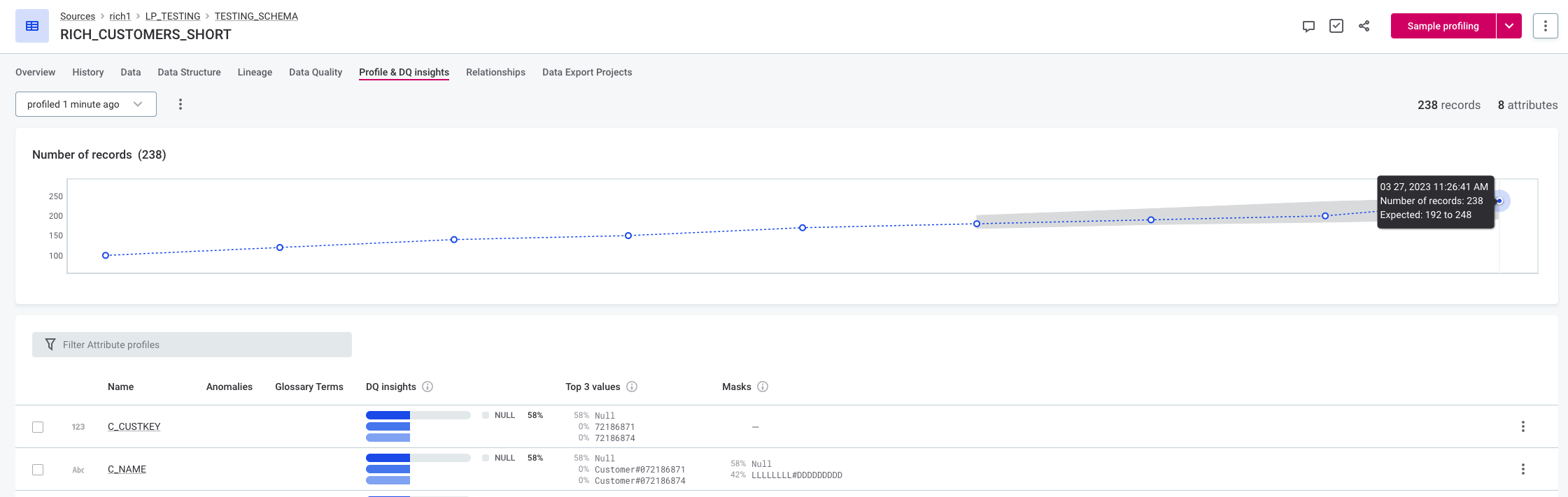
Changing the sensitivity for the time-dependent model also influences the extent of the expected range (the area highlighted in gray on the graph). For example, in the following figures the expected range with medium sensitivity is 200 to 239, but with low sensitivity the expected range is 192 to 248.

To select the anomaly detection sensitivity you want to use in profiling:

Select Global Settings > Profiling, and after selecting the required profiling configuration, select Edit.
In Anomaly detection sensitivity, select Very high, High, Medium, Low, or Very low.

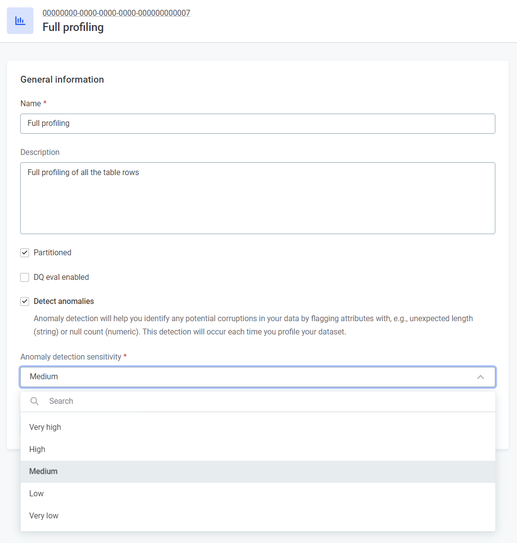
The Document flow uses full profiling, so to define the anomaly detection sensitivity of the Document flow, edit the sensitivity of Full profiling.

Exceptions

Some anomalies are detected regardless of sensitivity levels:

If an attribute did not contain any null values for at least the last five profiles, and now displays such values, it is flagged as anomalous.
If an attribute was positive in at least the last five profiles, and now displays zero or negative values, it is flagged as anomalous.
If an attribute was negative in at least the last five profiles, and now displays zero or positive values, it is flagged as anomalous.
If the number of records in a dataset has exhibited a consistent upward trend and suddenly begins to stagnate or decrease, it is flagged as an anomaly.

Run anomaly detection

To run anomaly detection on catalog items:

In Data Catalog > Catalog Items, select the required item.
Use the dropdown to select Full profiling or Full profile & DQ Evaluation.

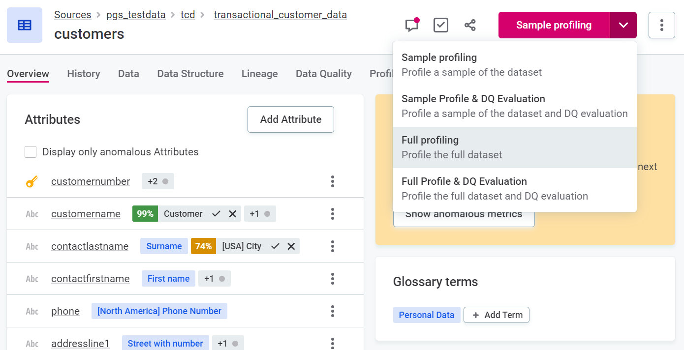
If custom profilings have been added which include anomaly detection, you can also select one of these. For more information, see Configure Profiling.

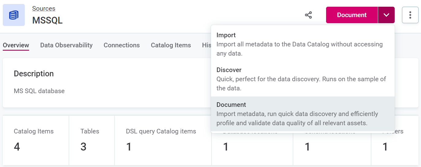
To run anomaly detection on sources:

In Data Catalog > Sources, select the required source.
Use the dropdown to select the Document documentation flow.

Detected anomalies

The presence of anomalies is marked using the warning icon. You can see information about any potential anomalies detected during profiling at a number of points in the Data Catalog:

Catalog item list view.
Attribute list view within a catalog item.

You can choose to view only the anomalous attributes of a catalog item by selecting Display only anomalous attributes.
In the Relationships and Lineage graphs (if Show Anomalies is selected in graph settings, see Configure Graph Style).
On the Profile and DQ Insights tab of a catalog item or attribute.

You can also view an aggregated list of all the catalog items with detected anomalies on the Anomaly Overview screen:

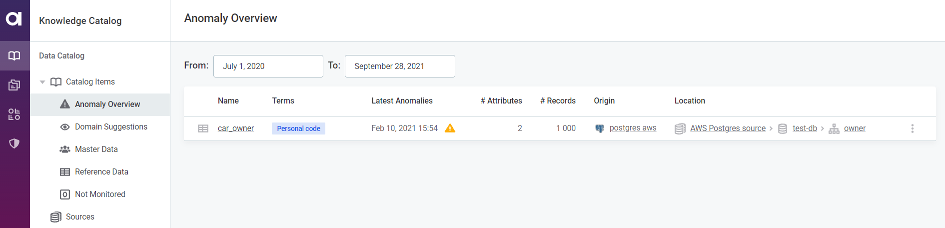
You can filter the detected anomalies according to a date range. If no date is provided in the To field, the current date applies.

Note that with the time-dependent model, an expected range is shown in gray, but no expected range is generated for the time-independent model.

View anomalous metrics

To view the metrics in the catalog item or attribute which are considered anomalous, open the Profile Inspector.

There are two ways to do this depending on where in the Data Catalog you see the detected anomaly information:

Select Show anomalous metrics.
Click the warning icon directly.

Profile inspector

Once you have opened the profile inspector, you can select whether you would like to view only anomalous items and metrics, or all, by using the Display only anomalous items and Display only anomalous metrics, respectively.

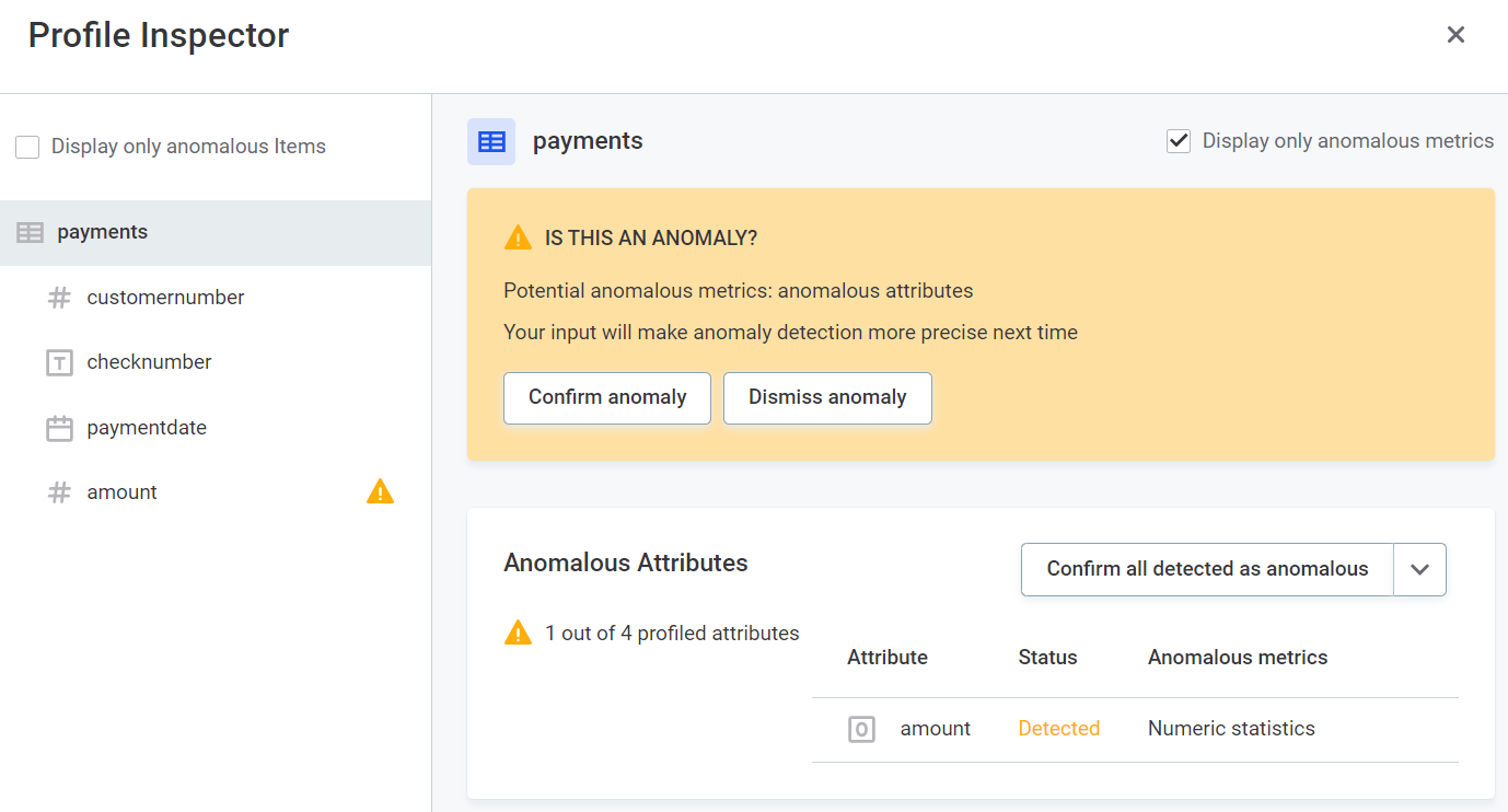
Before confirming or dismissing the anomaly, you can view the metrics in detail.

Catalog item metrics

Number of records: the number of records in the catalog item is checked with every profiling.

The gray background in the chart indicates the expected range of the values. Hover over the data points on the chart to see more details.

Attribute metrics

The anomalous results for a particular metric are shown over time with the highlighted outliers. Hover over the points on the chart to see more details such as values, profiling versions, and time.

Number of records
Mean
Minimum
Standard deviation
Numeric sum
Variance
Distinct count
Duplicate count
Non-unique count
Null count
Maximum
Unique count
Frequency, masks, and patterns

Ignored and missing timestamps

If time-dependent anomaly detection is being used, and no periodicity is specified, the system uses timestamps to derive periodicity.

Timestamps which are outside of the schedule are detected and are not used in the anomaly detection algorithm. This is shown in the application as Ignored timestamp.
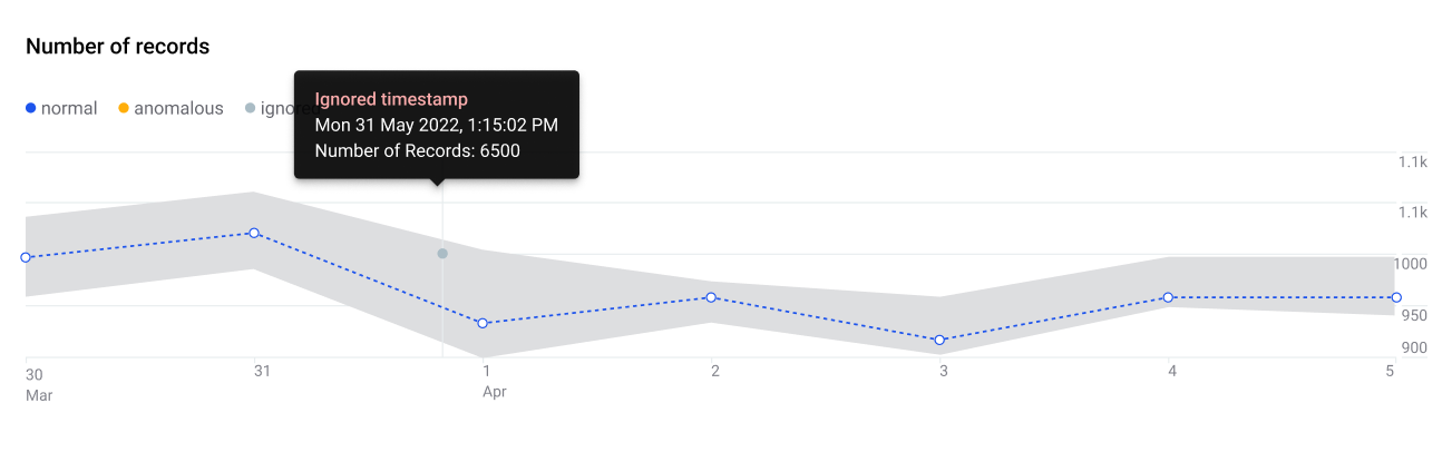
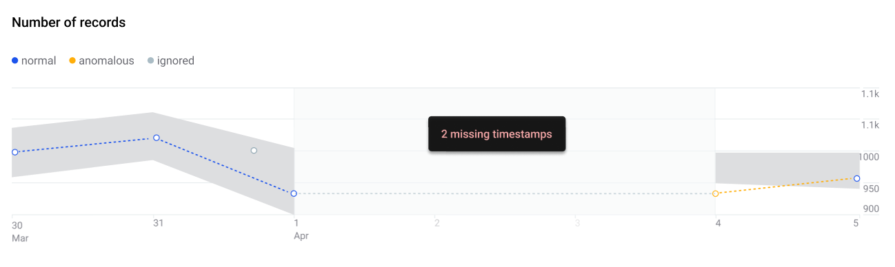
Timestamps which are missing are detected and the values are imputed for the purpose of anomaly detection. This is shown in the application as Missing timestamp.

Confirm or dismiss anomalies

Once anomalies have been detected, you can either confirm them or dismiss them. The anomaly detection model is constantly improved based on this user feedback.

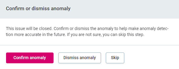
To do this:

Select the required catalog item or attribute in the Profile Inspector, and select Confirm anomaly or Dismiss Anomaly.
If an anomaly has been incorrectly confirmed or dismissed, select Review decision.

Confirm or dismiss all

In the Anomalous Attributes widget in Profile inspector, use the dropdown to select either Confirm all detected as anomalous or Dismiss all detected. Anomalies are confirmed or dismissed accordingly.

If an anomaly is dismissed on a particular attribute, this isn’t overridden if you subsequently select Confirm all detected as anomalous.

Unconfirmed anomalies

If detected anomalies are not confirmed, the system does not know to exclude them from the expected range. After some time (depending on the length of profiling history), the unsolved anomalies are considered the 'new normal', and a return to the expected values can subsequently be identified as anomalous.

How do I get anomaly detection to work for me?

Anomaly detection starts working from the 6th profile on, meaning that it is not activated for fewer profiles. This is the case for both models.

Furthermore, in case of higher periodicity, you might need even more profiles (at least twice the periodicity, that is, for periodicity 7, you need at least 14 profiles).

Choose your settings

There are a few questions which can help you determine which settings are appropriate for your use case:

Do you expect any trend, that is, increasing or decreasing of values over time?
Does your data increase in size, that is, adding new rows in each profile?
Do you expect periodic behavior, such as patterns that repeat daily or weekly?

If yes, select the time-dependent model.

Are there too many anomalies?

If yes, consider lowering the sensitivity of the algorithm in the profiling settings.

Are no anomalies being detected?

If yes, consider increasing the sensitivity of the algorithm in the profiling settings.

Is the model suggesting unsuitable anomalies?

If yes, consider changing the model.

It is possible that after a few rounds of profiling, you might realize that the selected model is not suitable for your particular use case. In such a scenario, you can change the selected model.

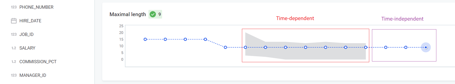
In the following figure, you can see two different models have been applied at various times.

Known limitations

An anomaly caused by variations in the number of records causes many other anomalies, particularly on count category (null-, distinct-, duplicate-, … count) in most of the attributes.
Anomalies are often detected on 'Frequencies' due to, for example:
- New keys appearing (this is an extreme case of random sample and is partially fixed).
- New keys added, lowering the relative occurrence of the existing keys.
Frequency keys are analyzed almost independently. It is not yet possible to reflect correlated changes among the keys.
The anomaly detection models start working optimally with more points, thus with few points it might be difficult to detect anomalies as expected.
The visualization might be confusing when switching between anomaly detection models (time-dependent and time-independent), as the time-dependent model shows the expected range while time-independent does not.
Anomaly detection rules are applied but an explanation of such rules not yet provided in the application. Anomaly detection rules aid or block detection of anomalies but no information about it is shown to the user, it has the same visualization as the anomaly detection models.

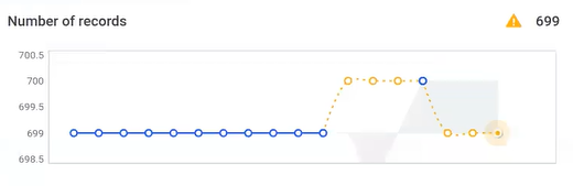
Feedback (confirm and dismiss)

Dismissing and confirming anomalies is important for the models to function optimally.

This example uses the time-independent model and the default sensitivity (medium). There is a jump in the number of records:

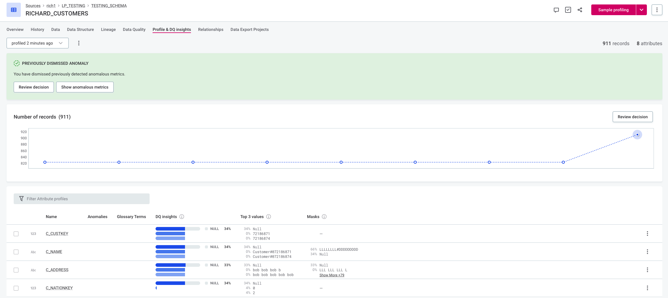
In the first instance, the algorithm detects it as an anomaly, but the user dismisses the suggestion. When the item is profiled again, the anomaly is no longer detected.
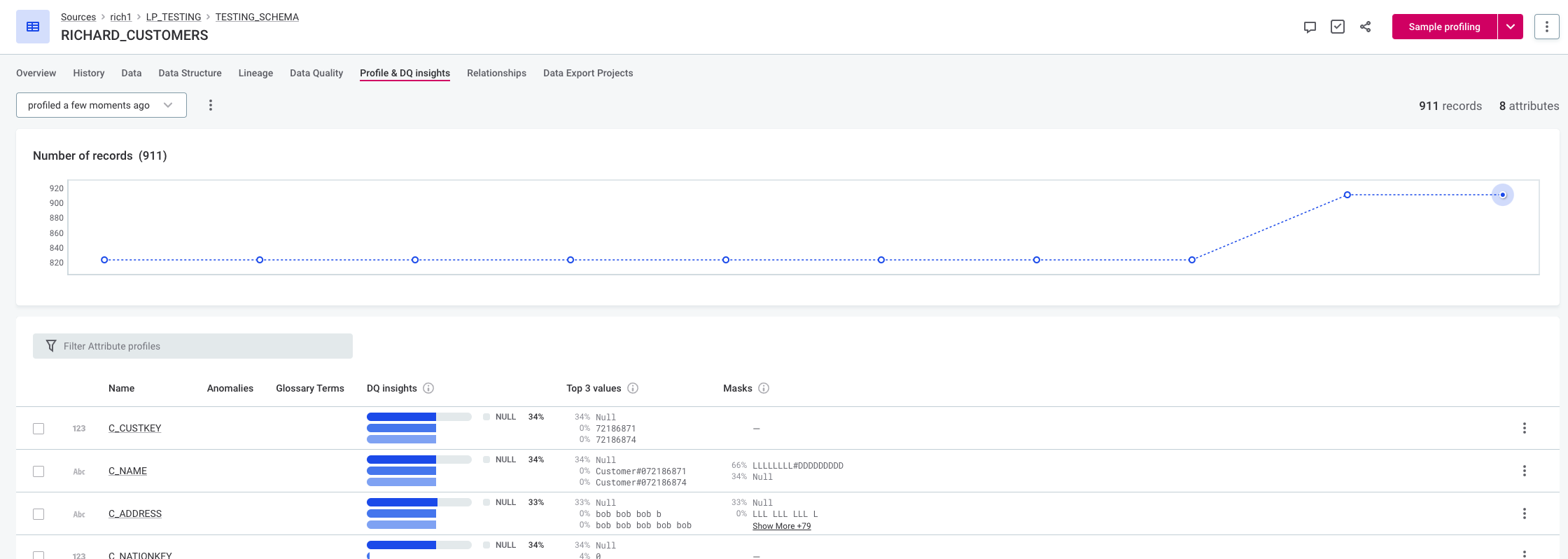
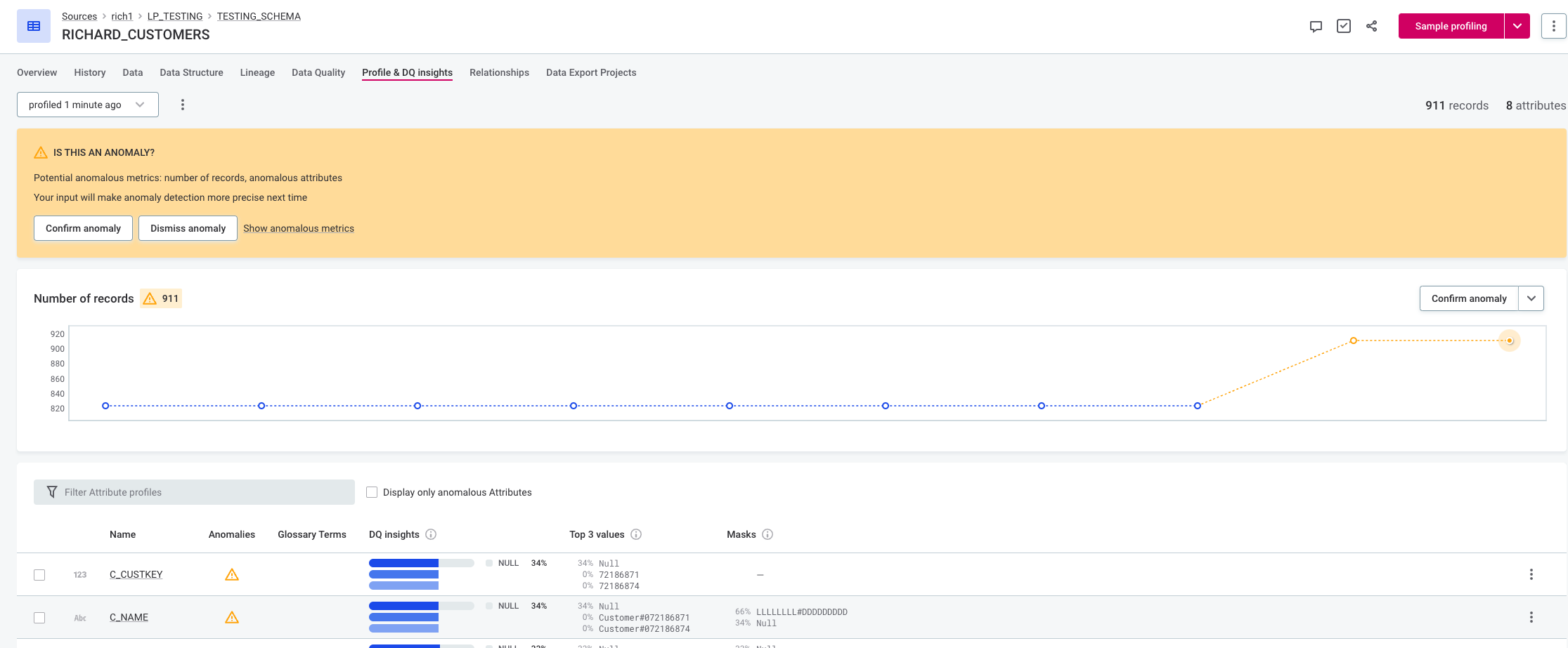
In the second instance, the user does not dismiss the anomaly. In this case the previous anomaly was not dismissed, and since the increase is very significant, the next value is also marked as anomalous.

Was this page useful?