
Time Series Data
Analysis of time series data can be carried out on all catalog items that contain at least one column with timestamp information: this can be either DATETIME, DATE, or DAY data types.
Time series analysis is designed to help you get the most from your transaction data, both in terms of identifying trends and detecting anomalies.
Transaction data describes an internal or external event or transaction that takes place in a business, and is most commonly associated with financial and logistical records. Examples include sales orders, invoices, purchase orders, shipping documents, document applications, payments, and insurance claims.
Benefits of time series analysis include:
-
Visual realization of time series data.
-
AI-driven anomaly detection.
Configure and run time series analysis
To get started:
-
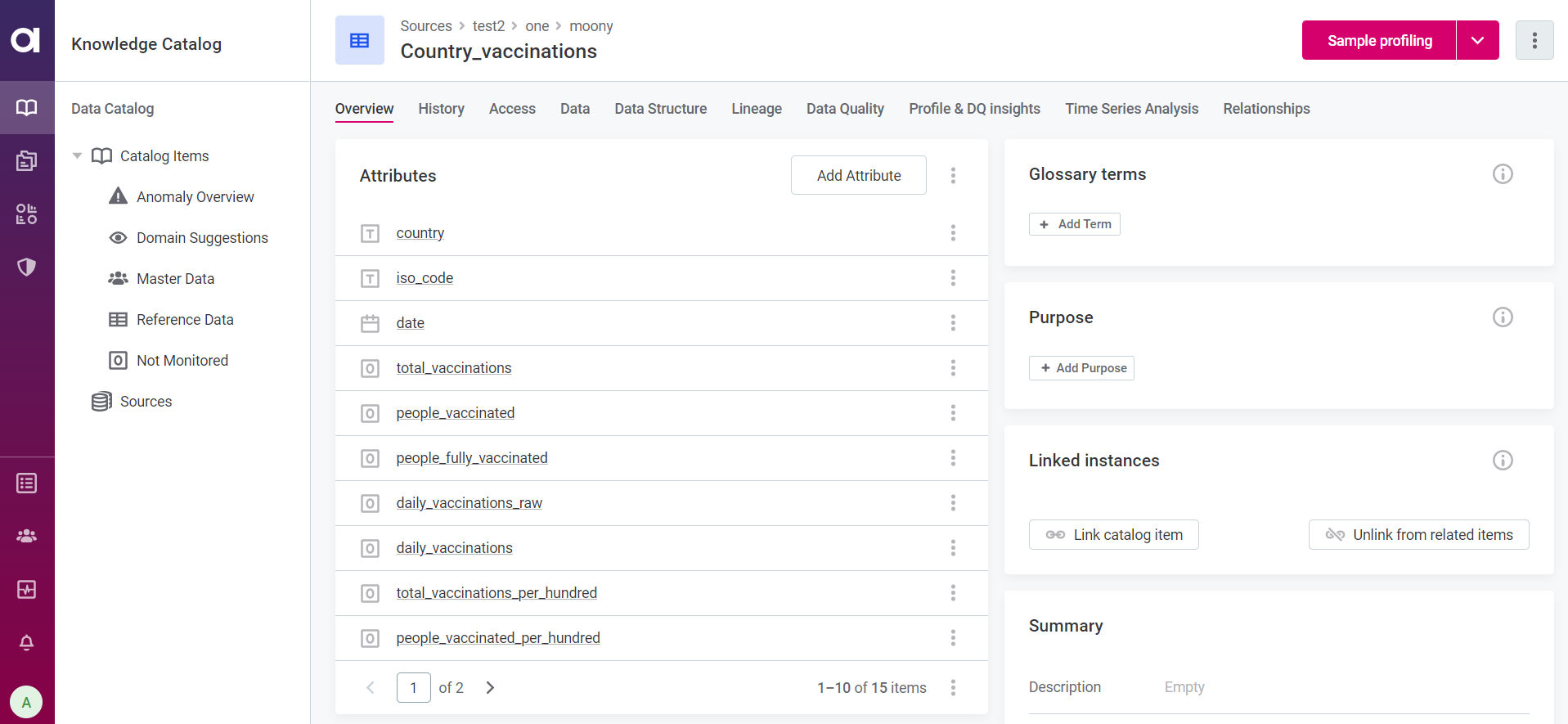
Navigate to Data Catalog > Catalog Items and select a catalog item of interest.
-
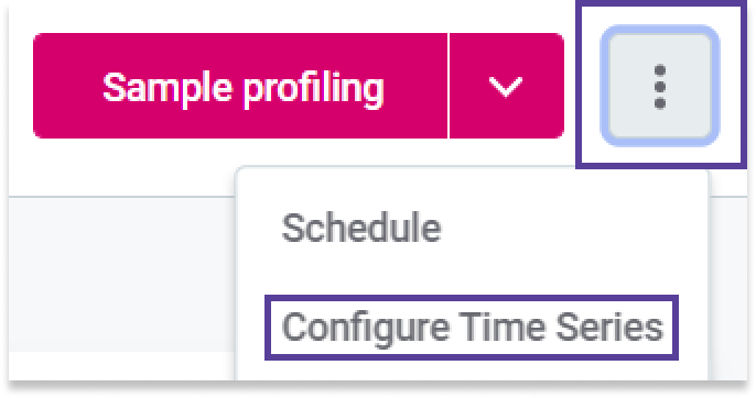
Use the three dots menu and select Configure Time Series.
-
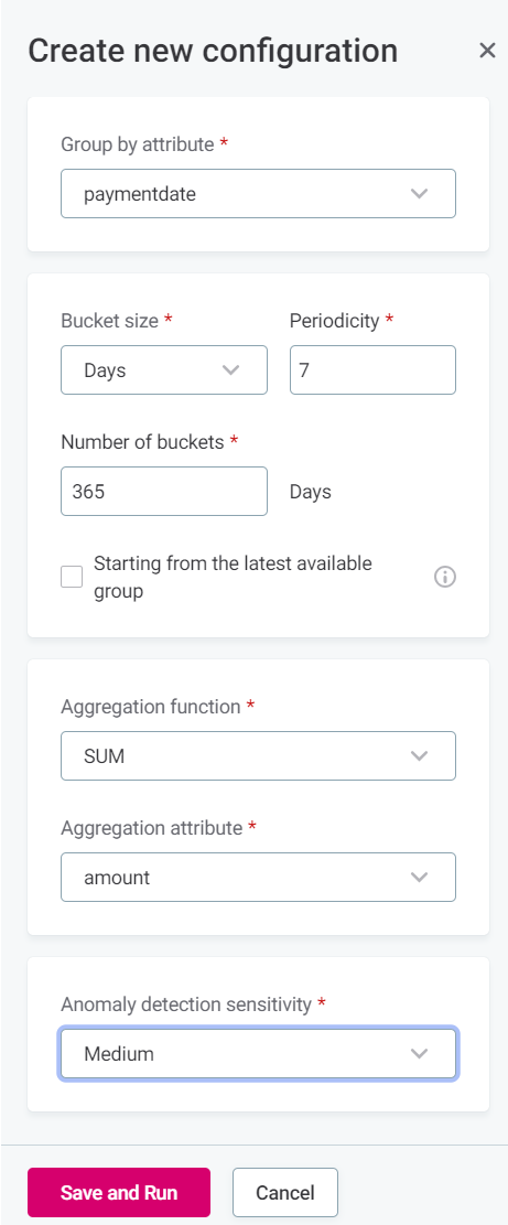
In the panel that opens, select Configure and fill in the following information:
-
Group by attribute: The catalog item attribute for which you want to run time series analysis.
-
Bucket size: Select how you would like to group the data from the Group by attribute. For example:
-
If you are interested in discovering hourly patterns such as 8 AM peaks or 6 PM drops, select Hours.
-
If you are interested in weekly patterns, such as how Monday data compares to Friday, select Days.
This works the same way as a
GROUP BYclause in SQL.The
GROUP BYstatement groups rows with the same values into summary rows. It is often used with aggregate functions (COUNT(),MAX(),MIN(),SUM(),AVG()) to group the result-set by one or more columns.
-
-
Periodicity: Periodicity of the underlying data.
The value suggested in this field is generated based on your selection in the Bucket size field; it is the optimal value for periodicity based on the selected grouping.
The suggested periodicity values are:
-
1: Most suitable when you are grouping the data by Years (a pattern repeating every one cycle of the selected grouping).
-
7: Most suitable when you are grouping by Days (a pattern repeating every seven cycles of the selected grouping).
-
12: Most suitable when you are grouping by Months (a pattern repeating every 12 cycles of the selected grouping).
-
24: Most suitable when you are grouping by Hours (a pattern repeating every 24 cycles of the selected grouping).
-
60: Most suitable when you are grouping by Minutes or Seconds (a pattern repeating every 60 cycles of the selected grouping).
You can adjust the suggested values according to your use case. For example, if there is a data point in the catalog item created every hour and you are expecting a pattern to repeat every two days, fill in Bucket size = Hours, Periodicity = 48.
-
-
Number of buckets: Select the window of data to be analyzed. For example, Bucket size = Days and Number of buckets = 365 analyzes data from the last 365 days.
The unit here reflects your selection in the Group by attribute field so it is not the same across all configurations. Make sure to note the unit specified. -
Starting from the latest available group: This option is useful when analyzing data that is no longer being collected, so its most recent groups are null.
Select this option to skip these null groups and start the window of time defined in Number of buckets from the last existing group.
-
Function: The aggregate function to be used. Available options are: SUM, COUNT, AVG, MIN, and MAX.
-
Aggregation attribute: The attribute you would like to aggregate by.
For example, if you would like to see hourly sales data, you would group by Hours and the aggregation attribute would be the column with the information on number of sales.
-
Anomaly detection sensitivity: Select from Very high, High, Medium, Low, and Very low.
High sensitivity means more points might be detected as anomalous but can result in false positives. Low sensitivity reduces the total number of anomalies detected but can result in false negatives.
Sensitivity in this context is measured as the number of standard deviations from the mean after which a point is considered as anomalous. The five options available correlate to the following values:
-
Very low: 4.5.
-
Low: 4.0.
-
Medium: 3.5.
-
High: 3.0.
-
Very high: 2.5.
This means, for example, that with the chosen sensitivity as Medium, anything which is further than 3 and half standard deviations from the mean is marked as anomalous.
-
-
-
Select Save and Run.
Interpreting time series results
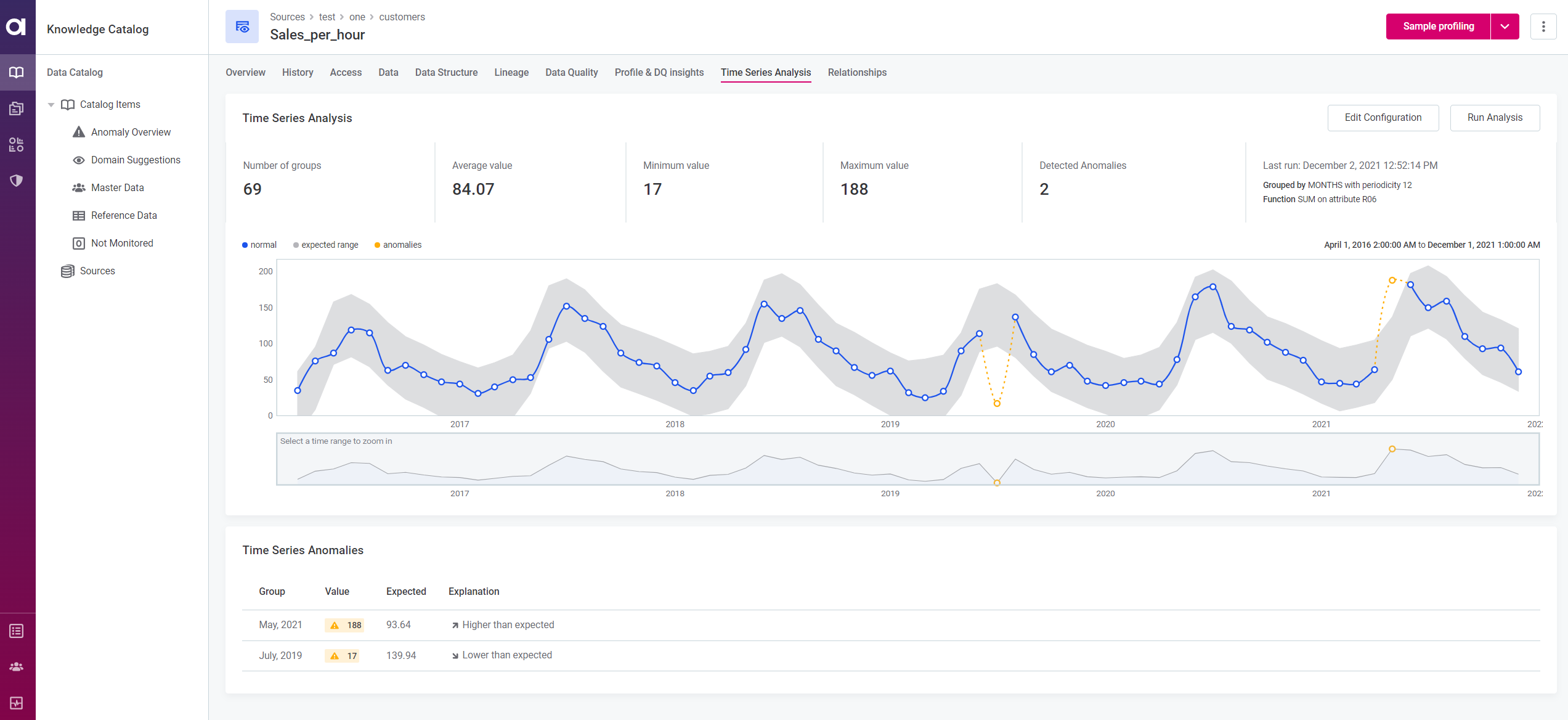
Outputs of time series analysis can be found under the Times Series Analysis tab of the catalog item, and include:
-
Key metrics of the data: Number of groups, Average value, Minimum value, Maximum value.
-
A graph displaying the data points, including anomalous points and the expected range.
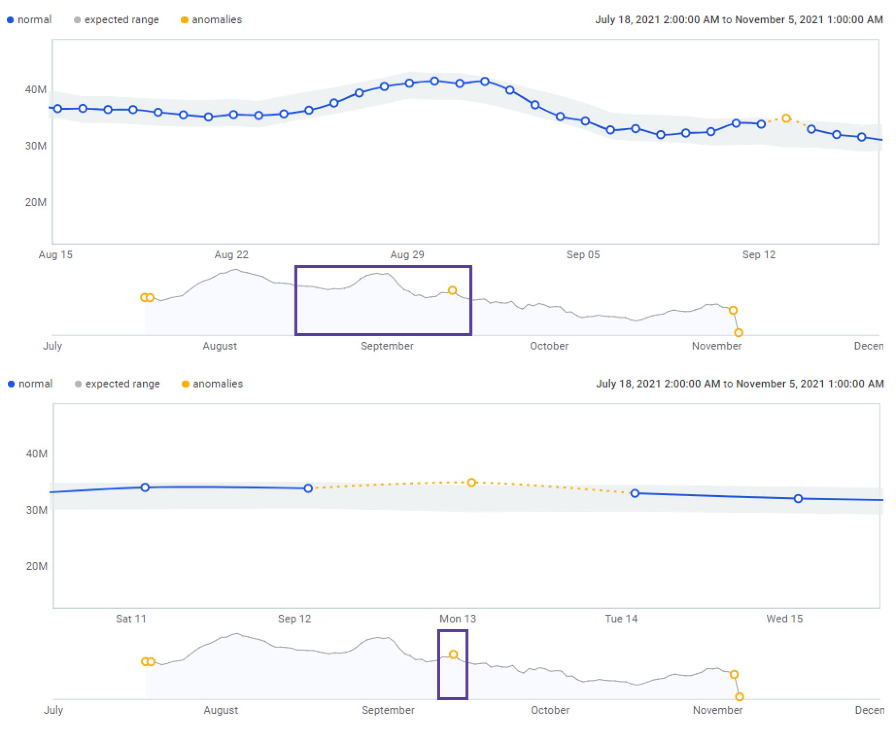
The second graph shows the full-time window specified. Move and resize the box to determine which results are shown on the primary graph. -
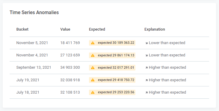
A list of anomalies, if detected, under Time Series Anomalies.
Anomaly detection is not available if there are not enough data points in the chosen time series configuration. For anomaly detection to be possible, the number of data points must be more than two times greater than the periodicity value, as well as greater than five.
For example, if the periodicity is seven, there needs to be at least 15 data points. If the periodicity is set to two, you need at least six data points.
Was this page useful?